Audit Data Analytics Part6

Backward stepwise regression

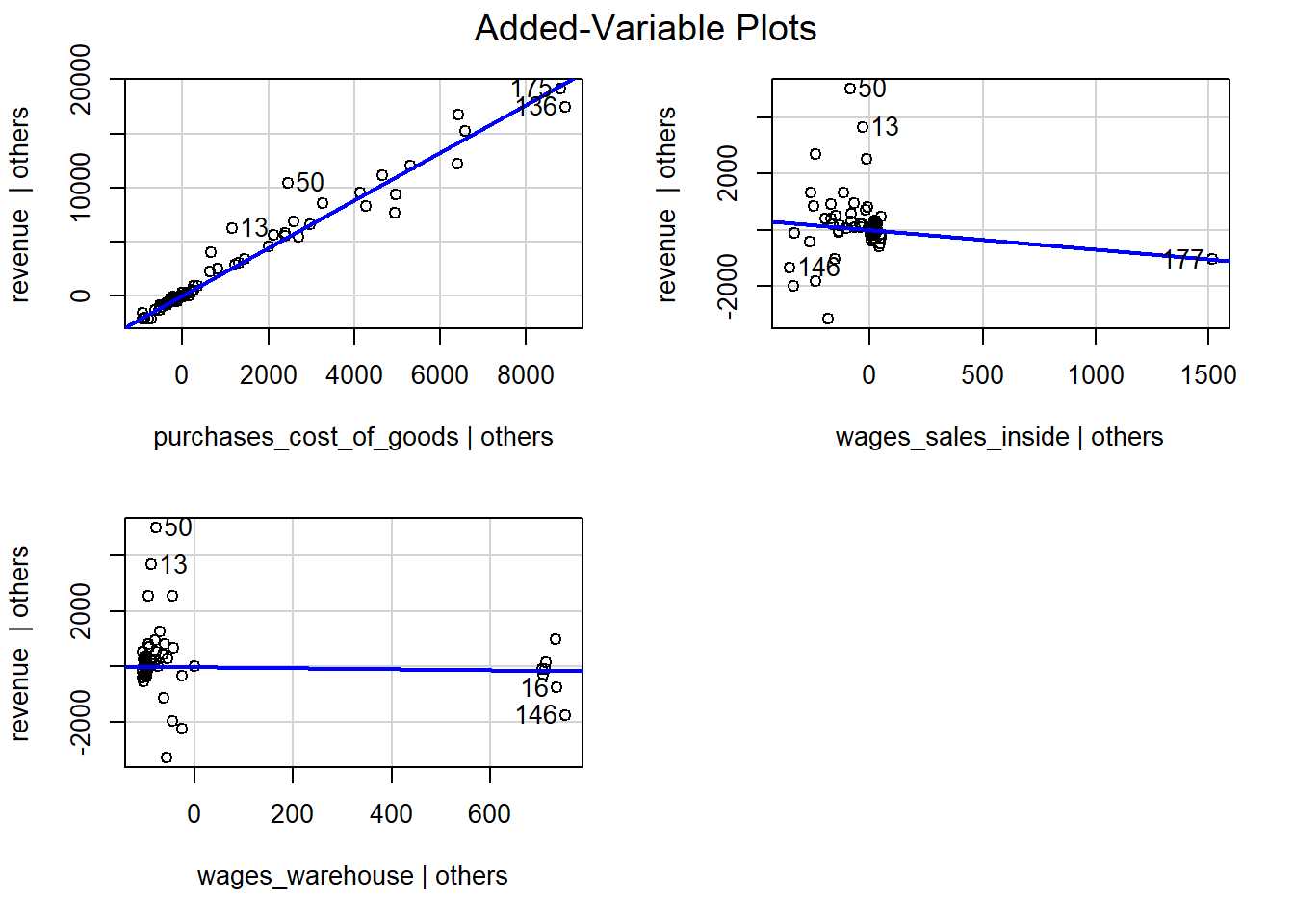
Three predictors selected by backward stepwise are purchases cost of goods, wages sales inside, and wages warehouse.

  Subset selection object
  Call: regsubsets.formula(revenue ~ ., data = df_model, nbest = 1, nvmax = 3, 
      method = "backward")
  11 Variables  (and intercept)
                           Forced in Forced out
  purchases_cost_of_goods      FALSE      FALSE
  wages_sales_inside           FALSE      FALSE
  payroll_tax_expenses         FALSE      FALSE
  wages_office_staff           FALSE      FALSE
  wages_warehouse              FALSE      FALSE
  conferences_and_seminars     FALSE      FALSE
  supplies                     FALSE      FALSE
  dues_and_subscriptions       FALSE      FALSE
  interest_expense             FALSE      FALSE
  maintenance_janitorial       FALSE      FALSE
  accounting_fees              FALSE      FALSE
  1 subsets of each size up to 3
  Selection Algorithm: backward

Linear regression

model_lm2 is selected after compared four lm models.

• model_lm vs model_lm1: no siginificant difference. One predictor (purchase) is sufficient.
  
• model_lm1 vs model_lm2: agrees to backward stepwise. Additional two predictors have some impact on target.
• model_lm1 vs model_lm3: different from random forest. Suggest interest expense and accoutning fees are not important.
• model_lm2 vs model_lm3: different from random forest. Interaction is not impactful.

  Analysis of Variance Table
  
  Model 1: revenue ~ purchases_cost_of_goods
  Model 2: revenue ~ purchases_cost_of_goods + wages_sales_inside + wages_warehouse
    Res.Df      RSS Df Sum of Sq      F  Pr(>F)  
  1    182 88558881                              
  2    180 84618271  2   3940610 4.1912 0.01663 *
  ---
  Signif. codes:  0 '***' 0.001 '**' 0.01 '*' 0.05 '.' 0.1 ' ' 1

  Analysis of Variance Table
  
  Model 1: revenue ~ purchases_cost_of_goods
  Model 2: revenue ~ purchases_cost_of_goods * interest_expense + accounting_fees
    Res.Df      RSS Df Sum of Sq      F Pr(>F)
  1    182 88558881                           
  2    179 88275037  3    283844 0.1919 0.9018

  Analysis of Variance Table
  
  Model 1: revenue ~ purchases_cost_of_goods + wages_sales_inside + wages_warehouse
  Model 2: revenue ~ purchases_cost_of_goods * interest_expense + accounting_fees
    Res.Df      RSS Df Sum of Sq F Pr(>F)
  1    180 84618271                      
  2    179 88275037  1  -3656766

                                 5 %        95 %
  (Intercept)              7.3369556 206.9033872
  purchases_cost_of_goods  2.1643745   2.2592575
  wages_sales_inside      -1.2743144  -0.1106398
  wages_warehouse         -0.5323339   0.1048621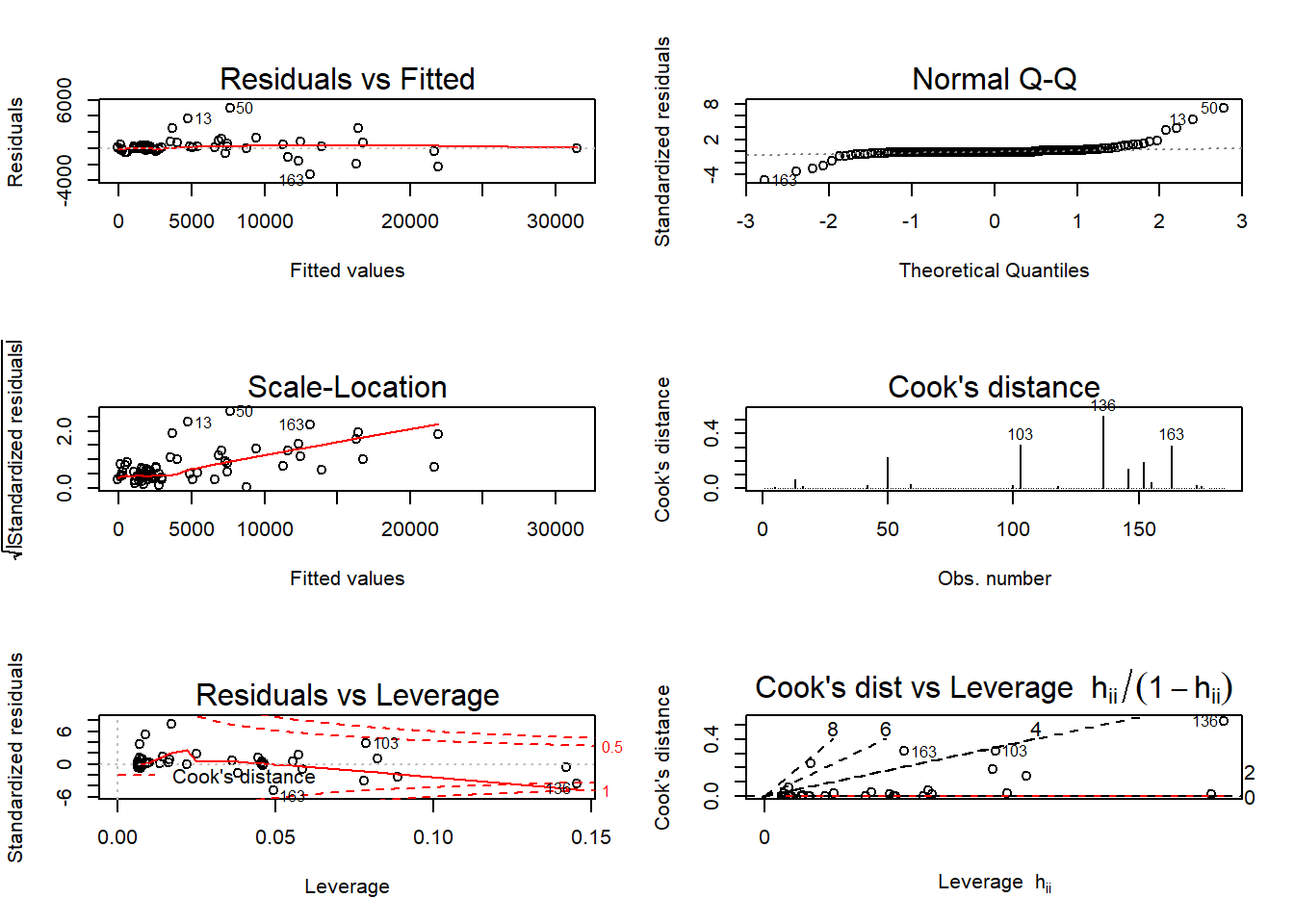

Model diagnostic

Assumptions

  
  Call:
  lm(formula = revenue ~ purchases_cost_of_goods + wages_sales_inside + 
      wages_warehouse, data = df_model)
  
  Residuals:
      Min      1Q  Median      3Q     Max 
  -3295.5  -107.1  -107.1    66.0  4972.7 
  
  Coefficients:
                           Estimate Std. Error t value Pr(>|t|)    
  (Intercept)             107.12017   60.35167   1.775   0.0776 .  
  purchases_cost_of_goods   2.21182    0.02869  77.083   <2e-16 ***
  wages_sales_inside       -0.69248    0.35191  -1.968   0.0506 .  
  wages_warehouse          -0.21374    0.19270  -1.109   0.2688    
  ---
  Signif. codes:  0 '***' 0.001 '**' 0.01 '*' 0.05 '.' 0.1 ' ' 1
  
  Residual standard error: 685.6 on 180 degrees of freedom
  Multiple R-squared:  0.9774,  Adjusted R-squared:  0.9771 
  F-statistic:  2600 on 3 and 180 DF,  p-value: < 2.2e-16
  
  
  ASSESSMENT OF THE LINEAR MODEL ASSUMPTIONS
  USING THE GLOBAL TEST ON 4 DEGREES-OF-FREEDOM:
  Level of Significance =  0.05 
  
  Call:
   gvlma::gvlma(x = model_lm2) 
  
                        Value   p-value                   Decision
  Global Stat        4559.600 0.000e+00 Assumptions NOT satisfied!
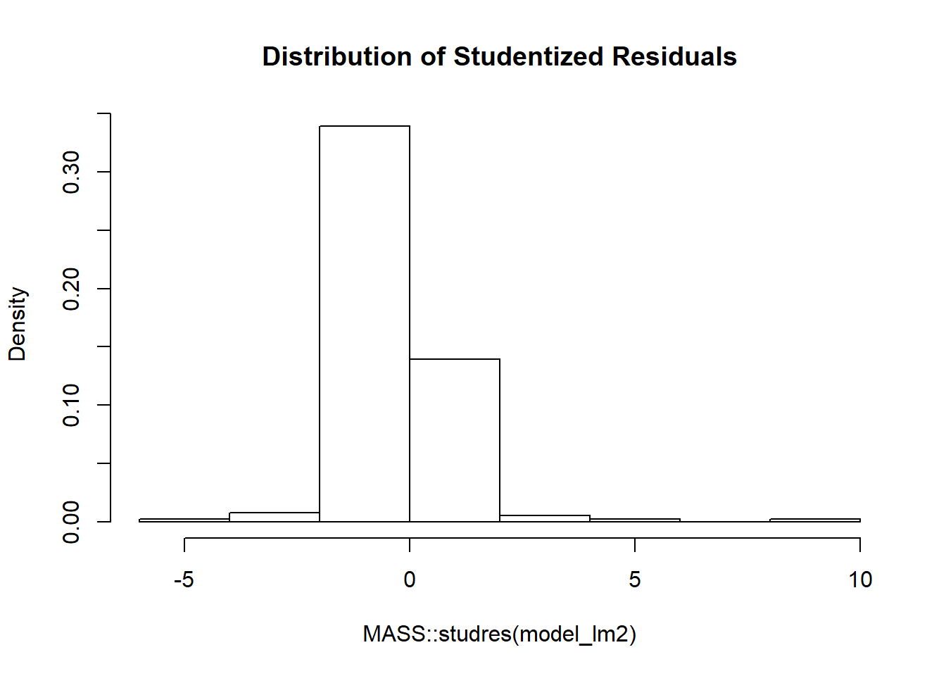
  Skewness            206.108 0.000e+00 Assumptions NOT satisfied!
  Kurtosis           4331.691 0.000e+00 Assumptions NOT satisfied!
  Link Function        19.572 9.689e-06 Assumptions NOT satisfied!
  Heteroscedasticity    2.229 1.354e-01    Assumptions acceptable.

Outliers

       rstudent unadjusted p-value Bonferroni p
  50   8.700994         2.1014e-15   3.8455e-13
  13   5.809475         2.8107e-08   5.1435e-06
  163 -5.285148         3.6238e-07   6.6316e-05
  103  3.999397         9.2791e-05   1.6981e-02
  100  3.799137         1.9878e-04   3.6377e-02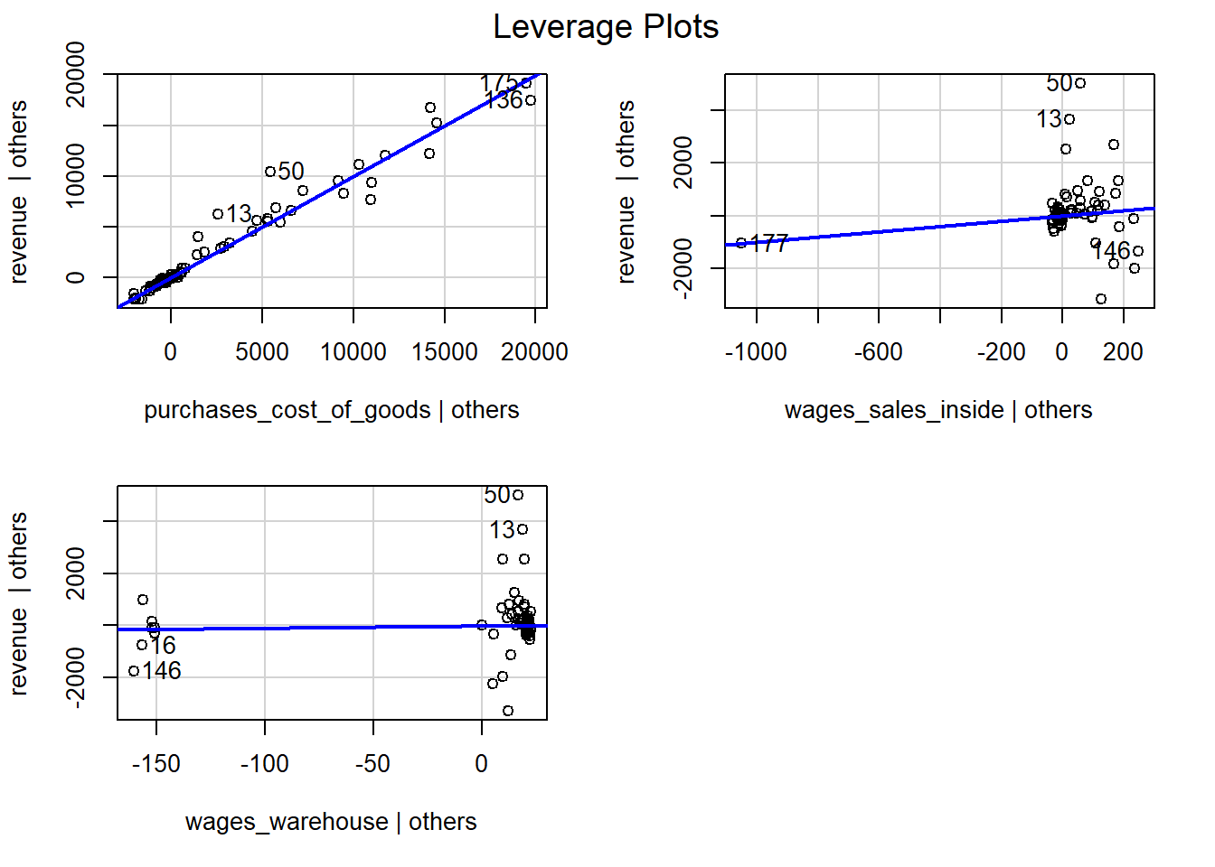

Influential Observations

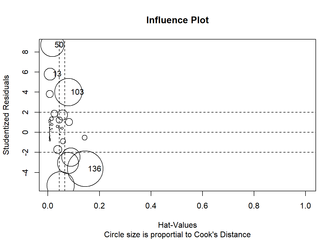
        StudRes         Hat      CookD
  13   5.809475 0.008581228 0.06178868
  50   8.700994 0.016838320 0.22907764
  103  3.999397 0.078728017 0.31544174
  136 -3.643572 0.145535897 0.52919937
  177       NaN 1.000000000        NaN

Normality of Residuals

Homoscedasticity

  
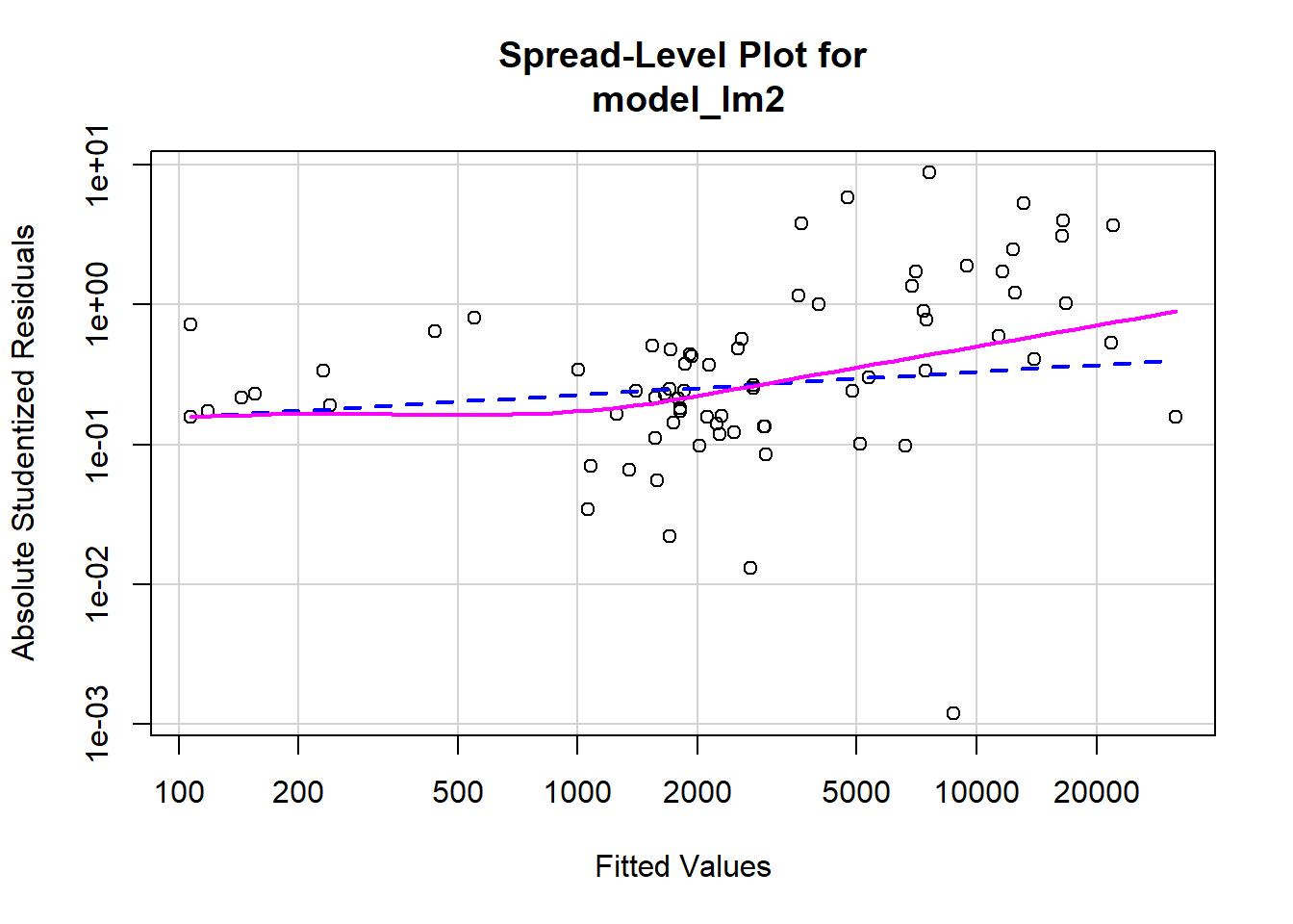
  Suggested power transformation:  0.8360112

Multicollinearity

kappa and vif are;

  [1] 278.8081

  purchases_cost_of_goods      wages_sales_inside         wages_warehouse 
                 1.356649                1.637527                1.254097

  [1] 1.416091

  purchases_cost_of_goods      wages_sales_inside         wages_warehouse 
                    FALSE                   FALSE                   FALSE

Nonlinearity

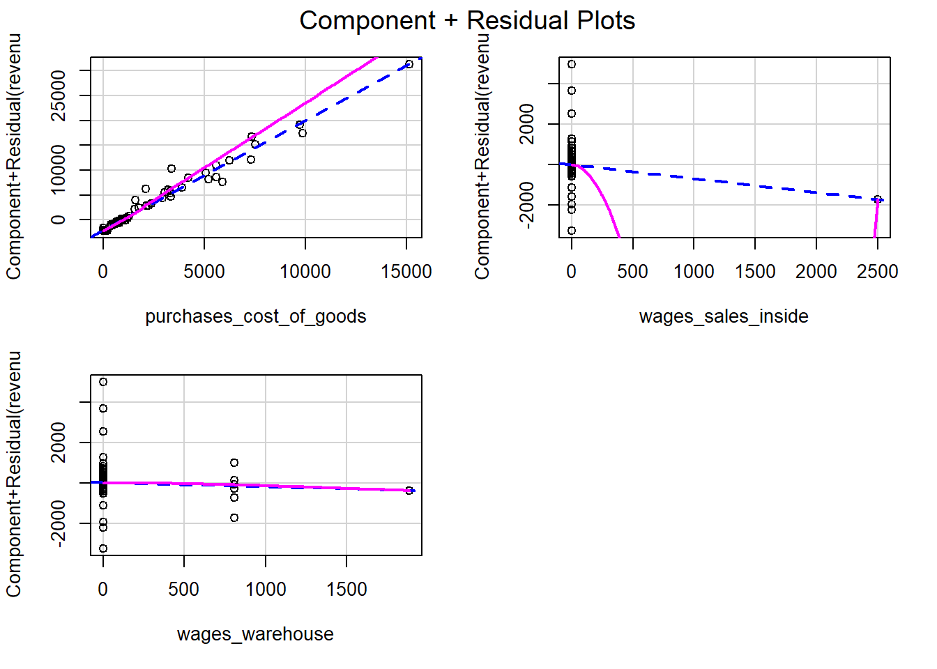
  Linear hypothesis test
  
  Hypothesis:
  purchases_cost_of_goods = 0
  wages_sales_inside = 0
  
  Model 1: restricted model
  Model 2: revenue ~ purchases_cost_of_goods + wages_sales_inside + wages_warehouse
  
  Note: Coefficient covariance matrix supplied.
  
    Res.Df Df      F    Pr(>F)    
  1    182                        
  2    180  2 9149.1 < 2.2e-16 ***
  ---
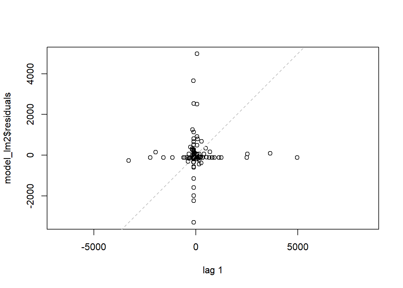
  Signif. codes:  0 '***' 0.001 '**' 0.01 '*' 0.05 '.' 0.1 ' ' 1

Autocorrelation

   lag Autocorrelation D-W Statistic
     1      0.01769898      1.964331
   Alternative hypothesis: rho0